Bioinformatics work notes
Navigating the Genome
-

Using AI to explain our research
Read More: Using AI to explain our researchTrying out AI to present scientific work as a podcast.
-

Unlocking Business Potential: Exploring the Value of External Bioinformatics Consultants
Read More: Unlocking Business Potential: Exploring the Value of External Bioinformatics ConsultantsHiring external consultants to handle or help with research and software development…
-
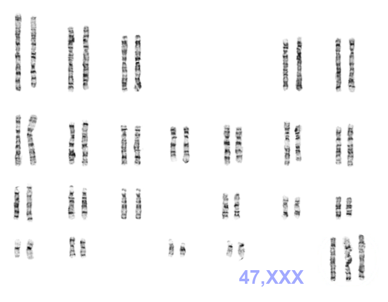
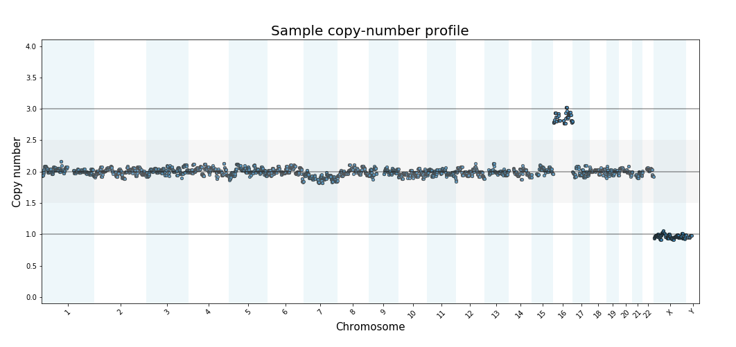
Common Whole-Chromosome Aneuploidies in Newborns
Read More: Common Whole-Chromosome Aneuploidies in NewbornsMost chromosome mis-segregation events lead to the death of the cell or…
-

SAM format summary
Read More: SAM format summaryThe Sequence Alignment/Map format as a generic alignment format for storing read…
-

Decoding REST: Simplifying Interconnected IT Systems
Read More: Decoding REST: Simplifying Interconnected IT SystemsRepresentational State Transfer to allow easy communication between systems over the internet.
-

Recover your wordpress site after your IP address has been blocked
Read More: Recover your wordpress site after your IP address has been blockedAccess the database to fix your broken website
-

Big Data with SQLite
Read More: Big Data with SQLiteUsing virtual tables to process genome-wide sequence data.
-
Read-counting for PGT-A
Read More: Read-counting for PGT-AIntroductory article about Pre-Implantation “Genetic Testing for Aneuploidy” using sequencing-based read-counting.
-

Microdeletion and Microduplication Syndromes in the Human Genome
Read More: Microdeletion and Microduplication Syndromes in the Human GenomeList of known Microdeletion and Microduplication Syndromes as of 2012
-

Website optimization
Read More: Website optimizationIdeas to improve specific parts of your web page.
-

CRAM format notes
Read More: CRAM format notesCRAM files are compressed versions of BAM files containing (aligned) sequencing reads.…
-

BlueFuse Multi Errors
Read More: BlueFuse Multi ErrorsA quick look-up for some of the BFM error codes.